WARLOCK ENGINEERING / INTERACTIVE RESEARCH WORKSPACE
Darrieus Engineering Notebook
Vertical-Axis Wind Turbine & Generator Research
YOU ARE VIEWINGStep 01 · Rotor aerodynamics
Swipe across the steps to see the complete notebook roadmap →
ENGINEERING NOTEBOOK / STEP 01 / RESEARCH ROTORS
Rotor aerodynamics.
Compare published rotor configurations, preserve the source evidence and explore their Cp–TSR curves.
YOUR ROTOR · SELECTED STUDY
See the rotor you are matching.
Watanabe et al. (2016) · NACA0024 straight blades. Choose the paper's blade count, chord and wind-lens configuration. The dimensions below are the tested reference.
Published rotor dimensions; schematic supports and theoretical NACA section, not measured profiles or fabrication CAD.
SECTION B / ADJUST AND COMPARE
Adjust and compare.
Choose a published rotor, adjust the supported settings and watch the Cp–TSR curve respond. The selection carries forward.
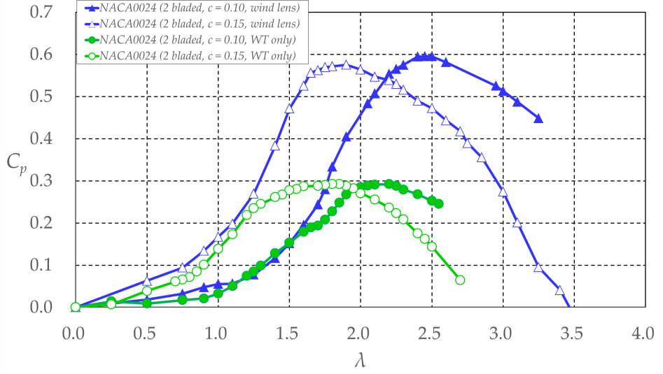
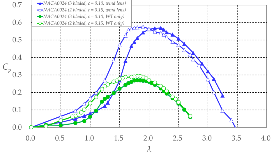
PERFORMANCE CURVE FIG. A
Power coefficient Cp vs. tip-speed ratio
ESTIMATED INTERPOLATION
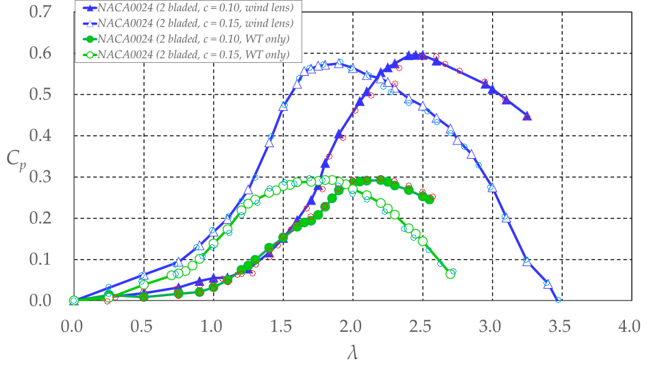
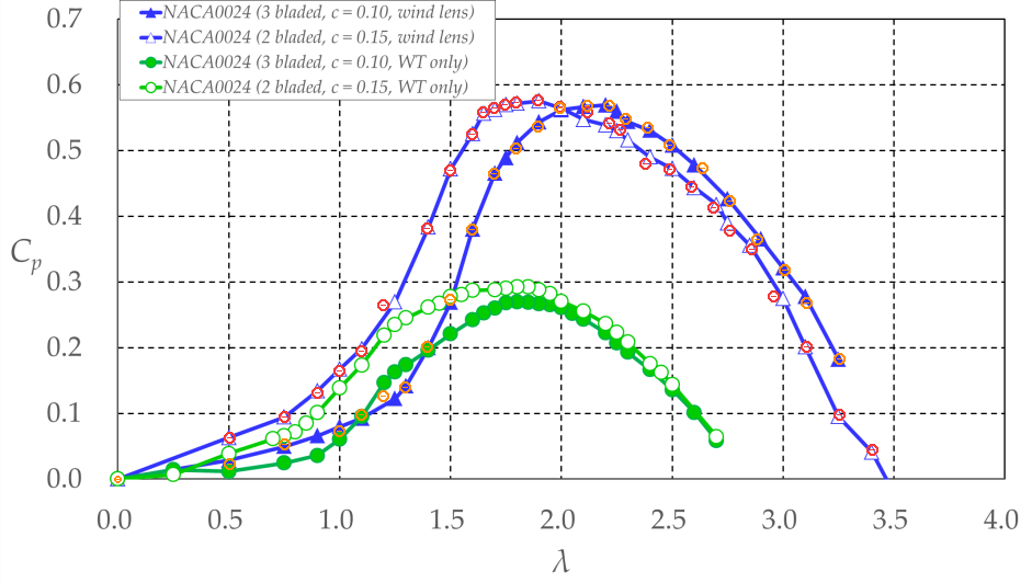
Bold line = selected rotor. Thin traces = measured reference chords. Small markers = digitised source points.
Li 2014 · experimental resonance: Figure 7 has no measurements at TSR 0.81–0.92 (about 132–149 RPM at 8.5 m/s). The dashed line is a visual connection only: those values remain unmeasured and unavailable for engineering calculations. Resonance may change with blade dimensions and supports.
Positive-power view is enlarged for readability. Battisti’s negative-Cₚ observations remain available above; at the roughly 400 RPM test condition these represent wind opposing the imposed rotation, not useful self-driven turbine output.
The evaluated TSR range is restricted to the available digitised measurements.
Method notes, published source details and graph artwork are provided for audit, not as additional experiments.
02 How the calculator works
I.
Evaluate the source curves
Each Figure 15 curve is traced with a monotone-preserving piecewise cubic interpolant (PCHIP) through its digitised points. No curve is extrapolated beyond its measured TSR range.
II.
Blend the curves at identical TSR (2 blades only)
t = (c − 100 mm) / (150 mm − 100 mm)
Cp(λ, c) = (1 − t)Cp,100(λ) + tCp,150(λ)
Changes in the peak TSR emerge from blending whole curves. We do not just shift one curve horizontally or vertically.
III.
Convert TSR to rotor RPM
RPM = 60 λ U / (π D)
RPM uses the paper's D = 0.70 m and U = 6.0 m/s. No generator loading is simulated in this module.
FIGURE 16 / PAGE 113 blades · 100 mm (fixed)WT only / wind lens · separate measured comparison
DATA QUALITY
These are visually approved digitised graph traces, not author-supplied raw measurements. Interpolated chords are estimates, not additional experiments.
PAPER DISCREPANCY
The Section 5 introduction lists wind-lens geometry L = 0.57D, φ = 20°, whereas the figure captions list L = 1.14D, φ = 15°. We have not resolved this conflict.
Inspect the source figure artwork and tracing overlays ⌄
Evidence distinction: Digitised traces are approximations of published plots. Interpolation stays within their supported domain; unknown startup behaviour and generator loading are not validated here.